Control Plots


The first page in the LLM + Control section where a plain prompt no longer suffices. The model cannot generate a plot — it can only emit text. So we give it three tools backed by python-control (root locus, Bode, Nyquist) and let it parse a natural-language request into numerator/denominator coefficient lists and call the matching tool. The model's job shifts from "do the math" to "translate the user's transfer function into tool inputs, then explain what the plot shows".
The three tools
Each wraps a python-control routine, renders the figure inline, saves a PNG, and returns a short text confirmation the model can read. Root locus shown here in full — Bode and Nyquist are the same shape (see the notebook for all three).
from pathlib import Path
import matplotlib.pyplot as plt
from control import root_locus, tf

PLOT_DIR = Path("plots")
PLOT_DIR.mkdir(exist_ok=True)


def plot_root_locus(numerator: list[float], denominator: list[float], title: str = "Root Locus") -> str:
    system = tf(numerator, denominator)
    fig, ax = plt.subplots(figsize=(6, 5))
    root_locus(system, ax=ax)
    ax.set_title(title)
    fig.savefig(PLOT_DIR / "root_locus.svg", bbox_inches="tight", dpi=120)
    plt.show()
    return f"Root locus rendered for numerator={numerator}, denominator={denominator}."
The tool schemas
All three schemas are parallel — same numerator / denominator / title parameters, only the name and description differ. One factory function keeps things dry:
def _schema(name: str, description: str) -> dict:
    return {
        "type": "function",
        "function": {
            "name": name,
            "description": description,
            "parameters": {
                "type": "object",
                "properties": {
                    "numerator":   {"type": "array", "items": {"type": "number"}},
                    "denominator": {"type": "array", "items": {"type": "number"}},
                    "title":       {"type": "string"},
                },
                "required": ["numerator", "denominator"],
            },
        },
    }


TOOL_SCHEMAS = [
    _schema("plot_root_locus", "Plot the root locus of a transfer function G(s) = N(s)/D(s)."),
    _schema("plot_bode",       "Plot the Bode magnitude and phase of a transfer function."),
    _schema("plot_nyquist",    "Plot the Nyquist diagram of a transfer function."),
]

TOOLS_BY_NAME = {
    "plot_root_locus": plot_root_locus,
    "plot_bode":       plot_bode,
    "plot_nyquist":    plot_nyquist,
}
The agent loop
Same five-line loop as Tool Use. Iterate chat.completions.create(..., tools=TOOL_SCHEMAS), execute any tool calls the model returns, feed the results back, stop when the model answers without a tool call:
import json

SYSTEM = (
    "You are a control-systems assistant with three plotting tools: "
    "plot_root_locus, plot_bode, and plot_nyquist. "
    "When the user gives you a transfer function G(s) = N(s)/D(s), "
    "parse N and D into polynomial coefficient lists in descending powers of s, "
    "then call the appropriate tool. "
    "After the tool runs, briefly describe what the plot shows."
)


def run_agent(user_message: str, max_steps: int = 5) -> str:
    messages = [
        {"role": "system", "content": SYSTEM},
        {"role": "user", "content": user_message},
    ]
    for _ in range(max_steps):
        resp = client.chat.completions.create(
            model=model,
            messages=messages,
            tools=TOOL_SCHEMAS,
            temperature=0,
        )
        msg = resp.choices[0].message
        messages.append(msg.model_dump(exclude_none=True))
        if not msg.tool_calls:
            return msg.content or ""
        for tc in msg.tool_calls:
            args = json.loads(tc.function.arguments or "{}")
            result = TOOLS_BY_NAME[tc.function.name](**args)
            messages.append({
                "role": "tool",
                "tool_call_id": tc.id,
                "content": result,
            })
    return messages[-1].get("content", "")
Example 1 — Root locus
The model parses the transfer function and calls the tool:
Model's commentary — qwen-plus (2026-04-21)
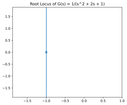
The root locus plot shows how the closed-loop poles of the system \(G(s) = \frac{1}{s^2 + 2s + 1}\) move in the complex plane as the gain \(K\) varies from 0 to \(\infty\). Since the denominator is \((s+1)^2\), the open-loop system has a double pole at \(s = -1\). For \(G(s) = \frac{K}{(s+1)^2}\), the characteristic equation is \(s^2 + 2s + 1 + K = 0 \Rightarrow s^2 + 2s + (1+K) = 0\), whose roots are \(s = -1 \pm j\sqrt{K}\). So the locus is a vertical line at \(\sigma = -1\), extending upward and downward as \(K\) increases.
This indicates the system remains stable for all \(K > 0\) (poles always have negative real part), but becomes increasingly underdamped with increasing \(K\).
Example 2 — Bode plot
Model's commentary — qwen-plus (2026-04-21)
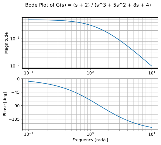
The Bode plot shows the frequency response of the transfer function \(G(s) = \frac{s + 2}{s^3 + 5s^2 + 8s + 4}\). It consists of two graphs:
- Magnitude plot — Shows the gain (in dB) versus frequency (log scale). The magnitude starts at approximately 6 dB at low frequencies and decreases at a rate of -40 dB/decade at high frequencies, indicating the system has three poles.
- Phase plot — Shows the phase shift (in degrees) versus frequency (log scale). The phase starts at 0° at low frequencies and approaches -90° at high frequencies, reflecting the dominant pole behavior.
Since this is a third-order system with all poles in the left half-plane, the system is stable. Gain margin and phase margin can be read from where the magnitude crosses 0 dB and where the phase crosses -180°.
Example 3 — Nyquist plot
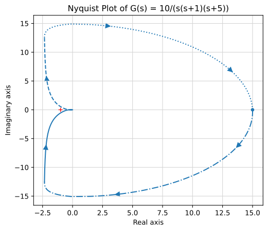
Notice the denominator is given in factored form. The model has to expand \(s(s+1)(s+5) = s^3 + 6s^2 + 5s\) before calling the tool — which it does, correctly:
Model's commentary — qwen-plus (2026-04-21)
The Nyquist plot traces the path of \(G(j\omega)\) as \(\omega\) varies. For this third-order system with three poles (at \(s = 0\), \(s = -1\), and \(s = -5\)) and no zeros, the plot:
- Starts at the origin (high-frequency gain goes to zero);
- Ends at the origin (as \(\omega \to \infty\));
- Approaches \(-270°\) of phase at high frequencies;
- Crosses the negative real axis, which matters for stability via the Nyquist criterion.
The plot helps determine closed-loop stability by examining how many times it encircles the critical point \((-1, 0)\).
Takeaways
The division of labor is clean:
- Model: natural-language → coefficient lists (including polynomial expansion when the user gives factored form), tool selection from the instruction, post-hoc analysis of the plot.
- Tool: everything numerical — transfer-function construction, frequency sweep, singular-value decomposition, plotting.
Neither alone is sufficient. A plain prompt could produce a textbook-style description of a Bode plot but no actual plot. A raw python-control call needs explicit coefficients, which is exactly the tedious step the model is now doing for you. This is the first rung on the staircase where the LLM and a deterministic tool each bring something the other cannot.
Next
Back to the LLM + Control overview, or forward to PID Tuning.